Project Overview
For my final project I explored simulating ocean's effieciently using procedural motion and dynamic level of detail. Some key algorithms and techniques I implemented include: fractional brownian motion (FBM) wave sampling, dynamic mesh upsampling/downsampling, and cubemap reflections .
FBM Wave Sampling
I explored several techniques for generating a realistic-looking ocean surface before landing on FBM. Some techniques that I considered included Gerstner waves and utilizing IFFT to transform wave spectra to the spatial domain for animating. I ended up choosing to use the nature of adding sine wave functions and FBM, as it provided good results and was not too complex to implement within the given time frame. To give an overview of the method, we can look at what superposition of sines really means.
The superposition of sines tells us that by adding multiple sine wave functions together, a new wave is produced, which holds the summation of each wave at that given point. This allows us to produce a complex displacement function by adding many wave samples with varying frequencies and amplitudes. This alone loses shape fast. If we take many, many samples with varying frequency and amplitudes in hopes of a realistic ocean, instead we get a chaotic mess as the waves have no limiting factor they approach.
Fractional Brownian Motion solves this issue by adding an external factor at each step. FBM does this by increasing the frequency and decreasing the amplitude by a set scaler at each step. This solves the issue by allowing finer and finer waves to be added at each step so that the amplitudes approach zero and don't cause chaotic mega waves.
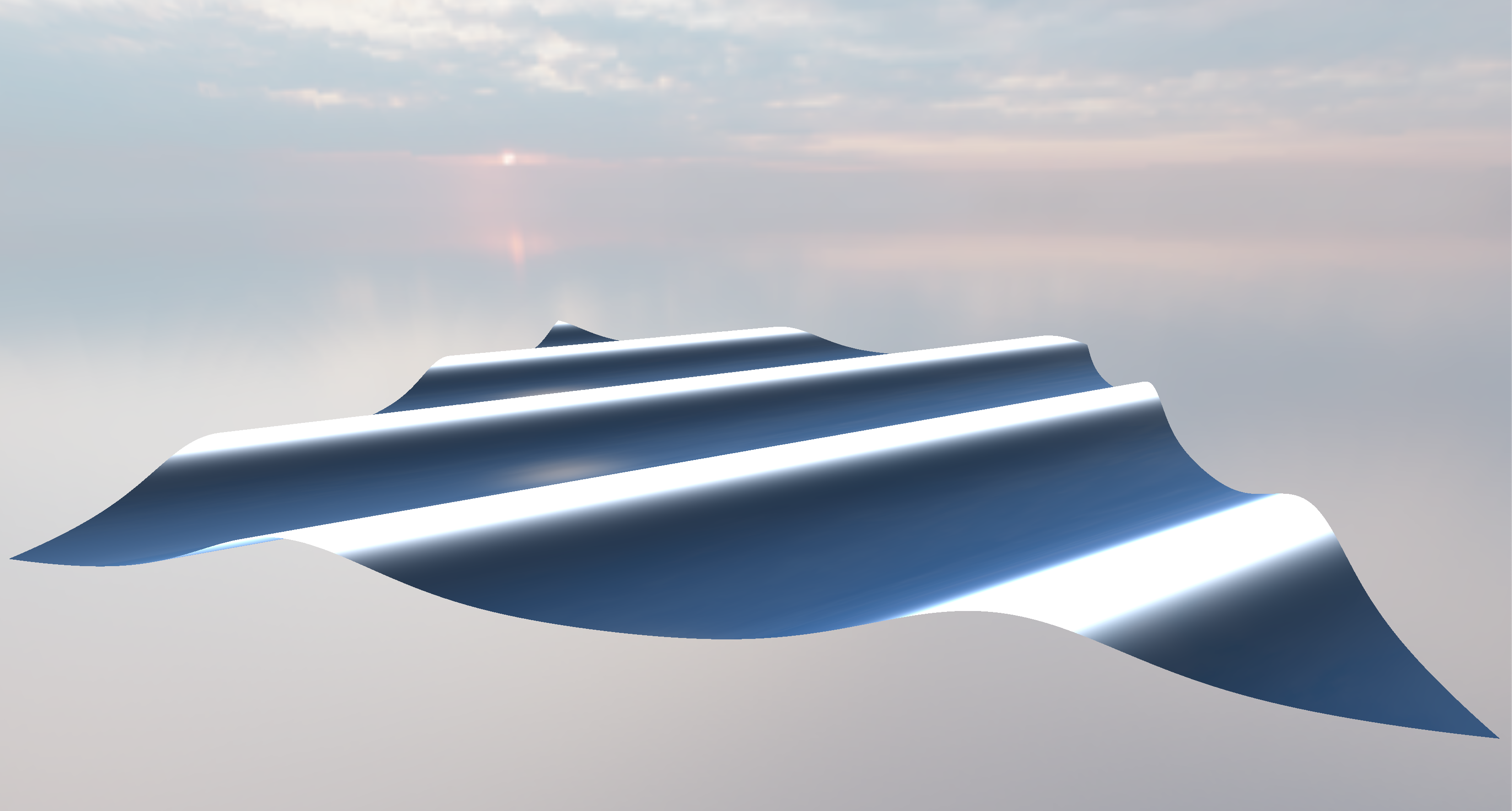
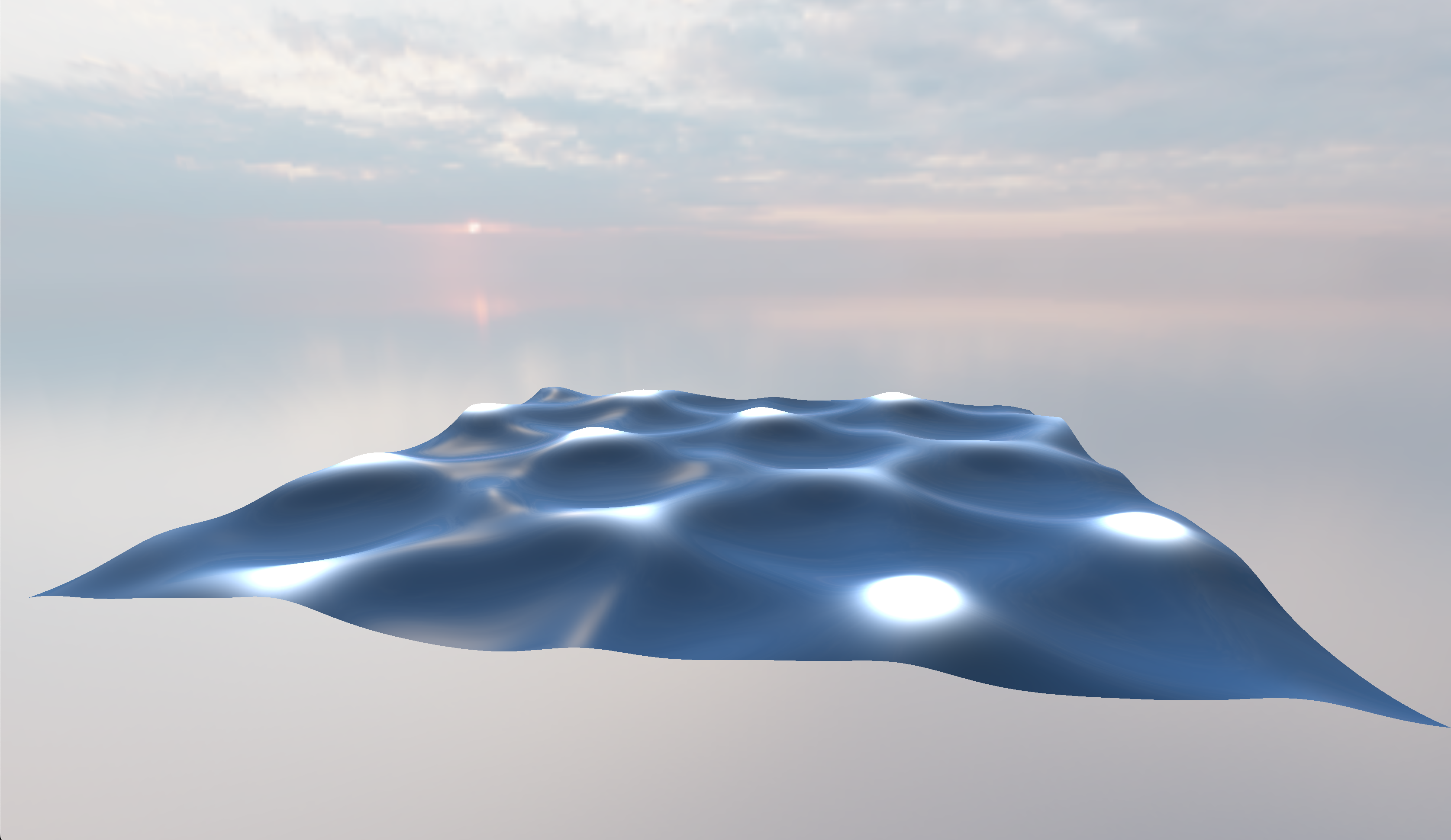
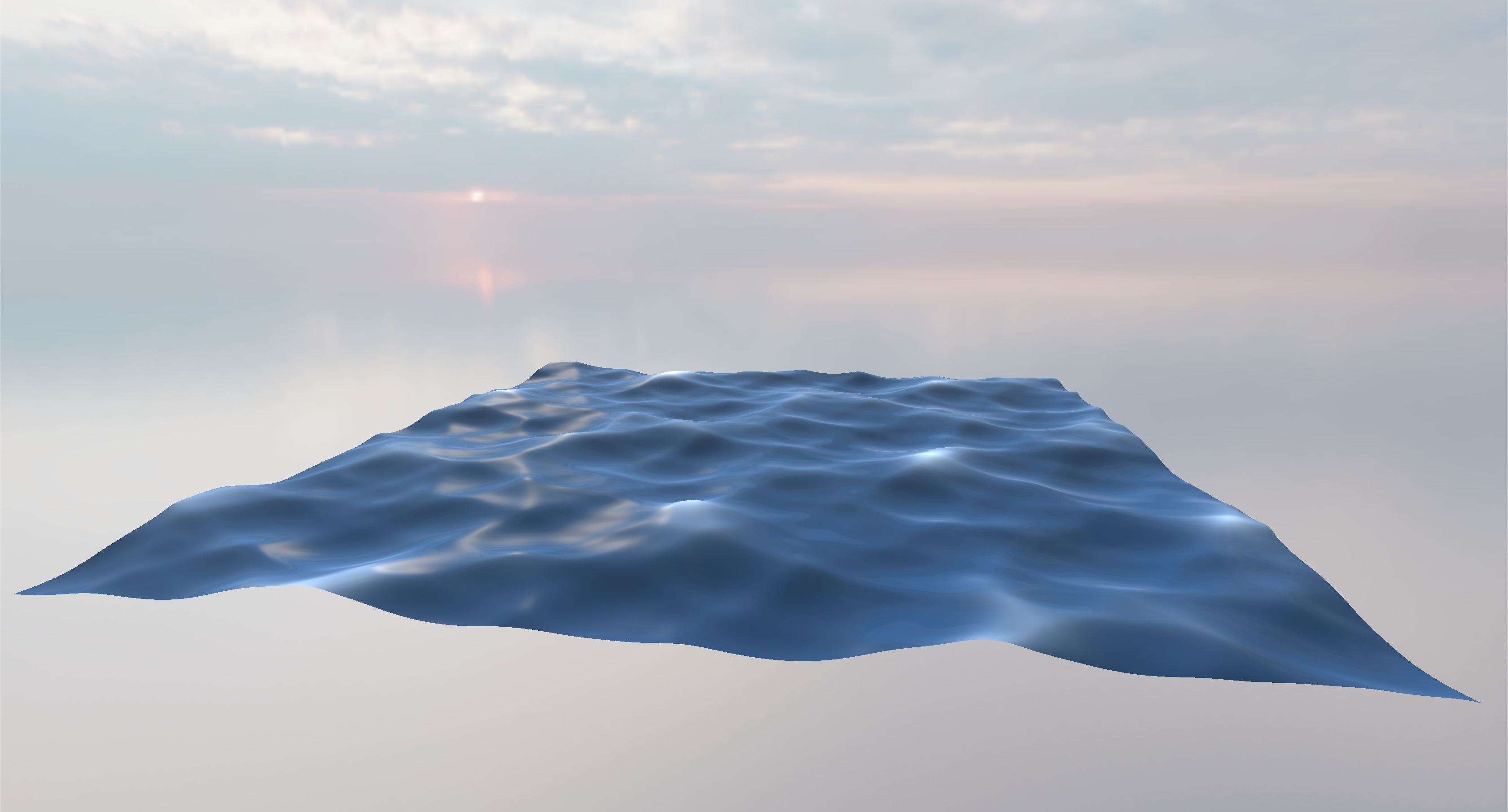
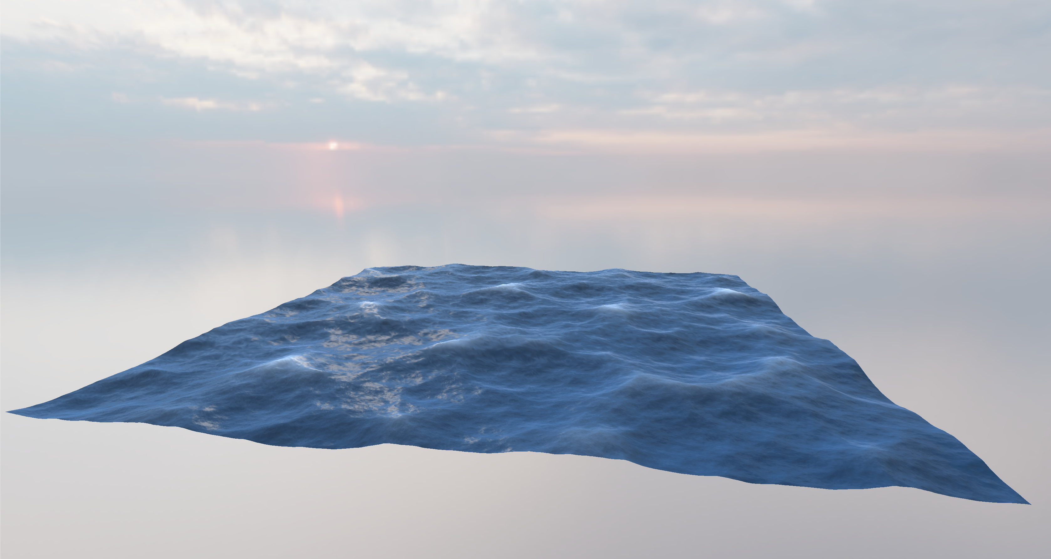
Fig 1. Wave Sample Iterations
Dynamic Level Of Detail
Dynamic level of detail was also added to the program to help with performance. Since each wave is being sampled around 64 times per vertex, this can add a lot of computation overhead on each draw call. With this in mind, I chose to explore the topic we discussed over the quarter relating to geometry manipulation via mesh upsampling and downsampling. This stage of the program was implemented using OpenGL's tessellation shader pipeline.
Tesselation shaders appear right after the geometry shader within the OpenGL rendering pipeline. They are an optional shader that allows us to perform subdivisions on the primitives generated after the vertex shader. There are three steps to this stage, two of which are programmable: Tesselation Control, Tesselation Primative Gen, and Tesselation Evaluation.
The tesselation control shader (TCS) is the first part of the process, this is where we determine how much tessellation to do. I utilized this shader to perform dynamic tesselation by interpolating between the camera-vertex distance for a tesselation level. This allowed for further patches to be simplified, and closer patches upsampled/subdivided.
After the intermediate points are generated, the tesselation evaluation shader (TES) evaluates these intermediate points to generate a new vertex point. It was within this shader that I sampled each newly created vertex and performed the FBM sum of sines process. Overall, with the dynamic LOD large ocean scenes could be rendered with wave sample counts of over 100 while not falling under 60fps.
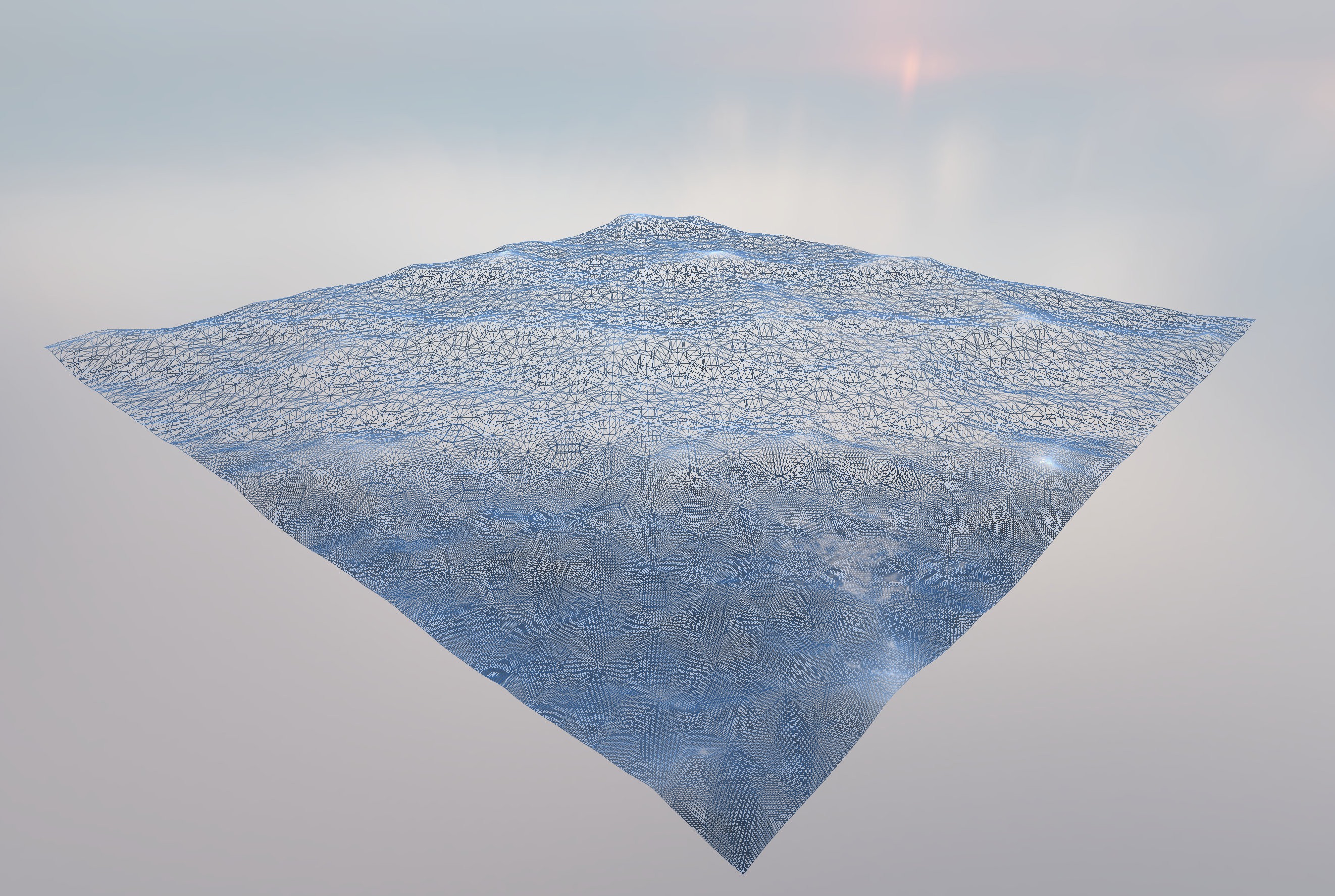
Fig 2. Wireframe Tesselation Example
Cubemap Reflections
For the water to be a little less strainous on the eyes I also added basic lighting techniques including cubemap reflections and fresnel. The cubemape based reflections work by sampling the reflected vector at each point from the camera onto the cubemap. This along with basic fresnel which makes things more reflective depending on the the angle of incidence helped sell the overall look of water. So as we get closer to the water and look down the horizon we get better water reflections and light shimmer.
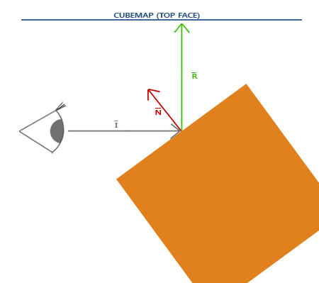
Fig 3. Cubemap reflection diagram
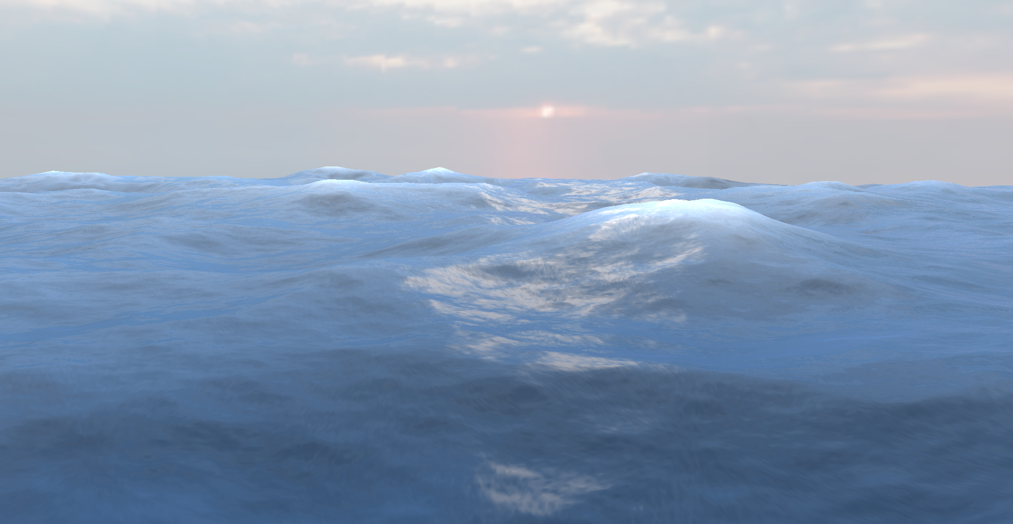
Fig 4. Example of high reflective incidence
Stylistically Customizable
With the many parameters that go into the wave sampling and calculations this also allowed for lots of stylistic control. With this capability, I was able to port the ocean to another scene pretty well.
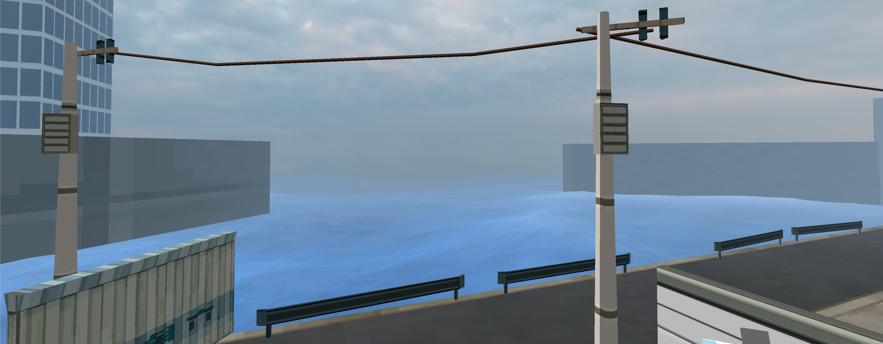
Fig 5. Ocean ported to harbor scene
References
- Fractional Brownian Motion basics: https://thebookofshaders.com/13/
- Project that went over lots of the math: https://helyum.it/projects/water-shader/
- Learning how Tesselation works: https://learnopengl.com/Guest-Articles/2021/Tessellation
- Original Paper to implement: https://dl.acm.org/doi/10.1145/3721239.3734101
- Acerolas video on topic: ://www.youtube.com/results?search_query=acerola+water